This page was generated from docs/notebooks/Reading and Writing transforms.ipynb.

%matplotlib inline

I/O - Reading and writing transforms

This notebook showcases the nitransforms.io module, which implements the input/output operations that allow this library to use other software packages’ formats and tools for transforms.

Preamble

Prepare a Python environment and use a temporal directory for the outputs. After that, fetch the actual file from NiBabel documentation.

import os
from pathlib import Path
from tempfile import TemporaryDirectory

import numpy as np
import nibabel as nb
import nitransforms as nt

cwd = TemporaryDirectory()
os.chdir(cwd.name)
print(f"This notebook is being executed under <{os.getcwd()}>.")

This notebook is being executed under </private/var/folders/l9/0lkn3g4s27bgkk75n6jj778r0000gp/T/tmpx7qowz2n>.

anat_file = Path(os.getenv("TEST_DATA_HOME", str(Path.home() / ".nitransforms"))) / "someones_anatomy.nii.gz"

Load in one sample image

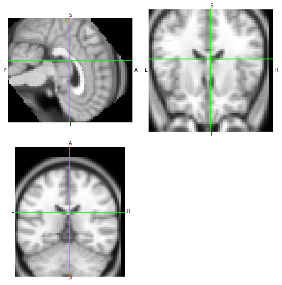
We pick NiBabel’s example dataset called someones_anatomy.nii.gz. This is a 3D T1-weighted MRI image stored in NIfTI format. Before any transformation, let’s first visualize the example image, and retain some copies of the original header and affine. Although it is not the only use-case for 3D images, most often when working with spatial transforms it is the case that at least one 3D image is involved.

Depending on how the software implements the functional that converts coordinates between two reference systems (which is, in essence, the transformation itself), the input/output images may play a role in defining said reference systems. The most common scenario where images are important to the definition of the spatial transform is that of image alignment (that is, resolving the image registration problem), where the algorithm works with the image’s array coordinates). Obviously, in such a framework, it is impossible to interpret any given transform without knowing the image(s) that define the real coordinates.

# Load the example
nii = nb.load(anat_file)
hdr = nii.header.copy()
aff = nii.affine.copy()
data = np.asanyarray(nii.dataobj)
nii.orthoview()

<OrthoSlicer3D: /Users/oesteban/datalad/nitransforms-tests/someones_anatomy.nii.gz (57, 67, 56)>

Image orientation

NIfTI images have two header entries to define how the data array indexed by integer coordinates between (0, 0, 0) and (\(S_i - 1\), \(S_j - 1\), \(S_k - 1\)) maps onto a continous space of, e.g., scanner coordinates (typically in mm). In order to ensure NiTransforms implements all possible combinations of transform formats and image orientations, we will need to generate similar images with different orientations.

To do so, we will use the nitransforms.tests.test_io._generate_reoriented(path, directions, swapaxes, parameters) function.

from nitransforms.tests.test_io import _generate_reoriented

For instance, we may want to generate an image in LAS orientation, where the first axis’ direction has been flipped and coordinates with positive sign get further away from the origin towards the left, rather than the right (i.e., RAS).

las_anatomy, _ = _generate_reoriented(anat_file, (-1, 1, 1), None, {"x": 0, "y": 0, "z": 0})
print(f"Orientation: {''.join(nb.aff2axcodes(las_anatomy.affine))}.")
print(f"Orientation of the original file: {''.join(nb.aff2axcodes(nii.affine))}.")

Orientation: LAS.
Orientation of the original file: RAS.

Because both orientations point to the same spatial mapping of T1w MRI measurements, with the LAS array having the first axis reversed, both images should look the same when visualized:

nii.orthoview()
las_anatomy.orthoview()

<OrthoSlicer3D: (57, 67, 56)>

Writing a rigid-body transform for AFNI, ANTs, and FSL

Now, let’s use these variants to check how they affect in concatenation with other transforms

First, we check that, as NiBabel represents the data array disregarding the affine, the .orthoview() visualization of the oblique image shows the same apparent data orientation as for the original file.

Create a transform. We test with a rigid-body transformation with 3 rotations and 3 translations

T = nb.affines.from_matvec(nb.eulerangles.euler2mat(x=0.9, y=0.001, z=0.001), [4.0, 2.0, -1.0])

Resampling the image with NiTransforms. Let’s resample the dataset using NiTransforms. We will be using the LAS image as reference, which means that it will define the output space, and the RAS conversion as moving image – where the actual values are drawn and moved from. This result should be similar with the other libraries.

xfm = nt.linear.Affine(T)
xfm.reference = las_anatomy

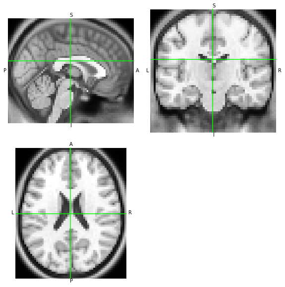
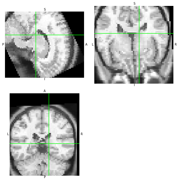
moved = xfm.apply(nii, order=0)
moved.to_filename('moved-nb.nii.gz')

moved.orthoview()

<OrthoSlicer3D: moved-nb.nii.gz (57, 67, 56)>

Store the transform in other formats. Let’s leverage NiTransforms’ features to store the transforms for ANTs, FSL, and AFNI. Because transforms can (generally) take any extension, for NiTransforms to know the format of the output we will need to inform the transform object’s method about the format with the fmt argument.

The transform object (xfm in this notebook) has a convenient method to_filename(). This method calls internally a factory class that assigns the correct type from nitransforms.io to correctly write out the output. to_filename() accepts a moving argument, and makes use of the reference property for those packages which require them (for example, FSL requires both, FreeSurfer LTAs writes their characteristics in the output file –although only necessary when the transform type is voxel-to-voxel,– and AFNI needs them only if the data array is not aligned with the cardinal axes –oblique).

xfm.to_filename('M.tfm', fmt='itk')
xfm.to_filename('M.fsl', moving=las_anatomy, fmt='fsl')  # reference is set in the xfm object
xfm.to_filename('M.afni', moving=las_anatomy, fmt='afni')  # reference is set in the xfm object
!ls

M.afni          M.fsl           M.tfm           moved-nb.nii.gz

The equivalent way of storing a transform using the low-level interface of the io submodule follows. Let’s store the transform T into FreeSurfer’s LTA format:

lta = nt.io.lta.FSLinearTransform.from_ras(T, moving=las_anatomy, reference=nii)
print(lta.to_string())

# LTA file created by NiTransforms
type      = 1
nxforms   = 1
mean      = 0.0000 0.0000 0.0000
sigma     = 1.0000
1 4 4
9.999990000003335e-01 1.404936252078656e-03 1.617172252089032e-04 -4.002644155280283e+00
-9.999993333334666e-04 6.216088741390577e-01 7.833271395738223e-01 -4.558906113709593e-01
9.999998333333415e-04 -7.833265179640611e-01 6.216096574657062e-01 2.184262694060495e+00
0.000000000000000e+00 0.000000000000000e+00 0.000000000000000e+00 1.000000000000000e+00
src volume info
valid = 1  # volume info valid
filename = /Users/oesteban/datalad/nitransforms-tests/someones_anatomy.nii.gz
volume = 57 67 56
voxelsize = 2.750000000000000e+00 2.750000000000000e+00 2.750000000000000e+00
xras   = 1.000000000000000e+00 0.000000000000000e+00 0.000000000000000e+00
yras   = 0.000000000000000e+00 1.000000000000000e+00 0.000000000000000e+00
zras   = 0.000000000000000e+00 0.000000000000000e+00 1.000000000000000e+00
cras   = 3.750000000000000e-01 1.125000000000000e+00 -1.400000000000000e+01
dst volume info
valid = 1  # volume info valid
filename = None
volume = 57 67 56
voxelsize = 2.750000000000000e+00 2.750000000000000e+00 2.750000000000000e+00
xras   = -1.000000000000000e+00 0.000000000000000e+00 0.000000000000000e+00
yras   = 0.000000000000000e+00 1.000000000000000e+00 0.000000000000000e+00
zras   = 0.000000000000000e+00 0.000000000000000e+00 1.000000000000000e+00
cras   = -2.375000000000000e+00 1.125000000000000e+00 -1.400000000000000e+01

Applying the transforms we generated before on images

Now, let’s check that the transforms written out by NiTransforms generate the same output as the tool generated with the apply() method when used with their corresponding software packages.

First, we will need to store a copy of our reference and moving images to the temporal directory where we are working:

nii.to_filename("someones_anatomy_RAS.nii.gz")
las_anatomy.to_filename("someones_anatomy_LAS.nii.gz")

The AFNI use-case. Let’s apply AFNI’s 3dAllineate to resample someones_anatomy_LAS.nii.gz into the grid of someones_anatomy_RAS.nii.gz through the affine we generated above:

!3dAllineate -base someones_anatomy_RAS.nii.gz -input someones_anatomy_LAS.nii.gz -1Dmatrix_apply M.afni -prefix moved-afni.nii.gz -final NN
moved_afni = nb.load('moved-afni.nii.gz')

++ 3dAllineate: AFNI version=AFNI_16.0.00 (Jan  1 2016) [64-bit]
++ Authored by: Zhark the Registrator
** AFNI converts NIFTI_datatype=2 (UINT8) in file someones_anatomy_RAS.nii.gz to FLOAT32
     Warnings of this type will be muted for this session.
     Set AFNI_NIFTI_TYPE_WARN to YES to see them all, NO to see none.
++ Source dataset: ./someones_anatomy_LAS.nii.gz
++ Base dataset:   ./someones_anatomy_RAS.nii.gz
++ You might want to use '-master' when using '-1D*_apply'
++ Loading datasets
++ NOTE: base and source coordinate systems have different handedness
 +       Orientations: base=Right handed (LPI); source=Left handed (RPI)
++ master dataset for output = base
++ OpenMP thread count = 4
++ ========== Applying transformation to 1 sub-bricks ==========
++ ========== sub-brick #0 ========== [total CPU to here=0.1 s]
++ Output dataset ./moved-afni.nii.gz
++ 3dAllineate: total CPU time = 0.1 sec  Elapsed = 0.1
++ ###########################################################

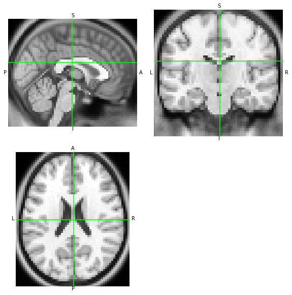
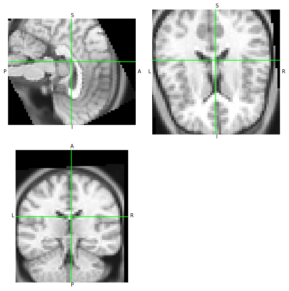
Now, the two resampled images –moved which we generated at the beginning using NiTransforms’ apply, and moved_afni just generated using 3dAllineate– should look the same.

moved.orthoview()
moved_afni.orthoview()

<OrthoSlicer3D: moved-afni.nii.gz (57, 67, 56)>

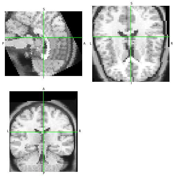
ANTs/ITK transforms. Similarly, let’s test antsApplyTransforms

!antsApplyTransforms -d 3 -i 'someones_anatomy_LAS.nii.gz' -r 'someones_anatomy_RAS.nii.gz' -o 'moved-itk.nii.gz' -n 'NearestNeighbor' -t 'M.tfm' --float
nb.load('moved-itk.nii.gz').orthoview()

<OrthoSlicer3D: moved-itk.nii.gz (57, 67, 56)>

FSL. Finally, let’s check with FSL flirt

!flirt -in someones_anatomy_LAS.nii.gz -ref someones_anatomy_RAS.nii.gz -out moved-fsl.nii.gz -init M.fsl -applyxfm
nb.load('moved-fsl.nii.gz').orthoview()

<OrthoSlicer3D: moved-fsl.nii.gz (57, 67, 56)>

The special case of oblique datasets and AFNI

AFNI implements spatial transforms in physical coordinates (mm), so it doesn’t generally require to know about the reference and moving images to calculate coordinate mappings (obviously, both are required when applying the transform to align one another).

Let’s use an oblique dataset rotated 0.2 rad around the X axis and 0.1 rad around Y for the reference image in this case.

oblique, _ = _generate_reoriented(anat_file, (1, 1, 1), None, {"x": 0.2, "y": 0.1, "z": 0})
print("Dataset is oblique" if nt.io.afni._is_oblique(oblique.affine) else "not oblique (?)")
oblique.to_filename("oblique.nii.gz")

Dataset is oblique

Let’s first check the contents of the output file when neither the reference nor the moving images were oblique:

nonoblique_M = nt.io.afni.AFNILinearTransform.from_ras(T, moving=las_anatomy, reference=nii)
print(nonoblique_M.to_string())

# 3dvolreg matrices (DICOM-to-DICOM, row-by-row):
0.999999        -0.000999999    -0.001  -4      0.00140494      0.621609        0.783327        -2      -0.000161717    -0.783327       0.62161 -1

Now, let’s replace the reference with the oblique image:

oblique_M = nt.io.afni.AFNILinearTransform.from_ras(T, moving=las_anatomy, reference=oblique)
oblique_M.to_filename("M.oblique.afni")
print(oblique_M.to_string())

# 3dvolreg matrices (DICOM-to-DICOM, row-by-row):
0.994885        -0.000781397    -0.101006       -13.492 0.0903701       0.453595        0.886614        12.7541 0.0451231       -0.891208       0.451346        -13.9663

It is apparent that the transform is not the same as above anymore. Let’s see whether AFNI interprets these new parameters correctly.

!3dAllineate -base oblique.nii.gz -input someones_anatomy_LAS.nii.gz -1Dmatrix_apply M.oblique.afni -prefix moved-afni-oblique.nii.gz -final NN
moved_afni = nb.load('moved-afni-oblique.nii.gz')

++ 3dAllineate: AFNI version=AFNI_16.0.00 (Jan  1 2016) [64-bit]
++ Authored by: Zhark the Registrator
*+ WARNING:   If you are performing spatial transformations on an oblique dset,
  such as oblique.nii.gz,
  or viewing/combining it with volumes of differing obliquity,
  you should consider running:
     3dWarp -deoblique
  on this and  other oblique datasets in the same session.
 See 3dWarp -help for details.
++ Oblique dataset:oblique.nii.gz is 12.794579 degrees from plumb.
++ Source dataset: ./someones_anatomy_LAS.nii.gz
++ Base dataset:   ./oblique.nii.gz
++ You might want to use '-master' when using '-1D*_apply'
++ Loading datasets
++ NOTE: base and source coordinate systems have different handedness
 +       Orientations: base=Right handed (LPI); source=Left handed (RPI)
++ master dataset for output = base
++ OpenMP thread count = 4
++ ========== Applying transformation to 1 sub-bricks ==========
++ ========== sub-brick #0 ========== [total CPU to here=0.1 s]
++ Output dataset ./moved-afni-oblique.nii.gz
++ 3dAllineate: total CPU time = 0.1 sec  Elapsed = 0.1
++ ###########################################################

Looking closely at the standard output of 3dAllineate we can spot that the dataset is correctly identified as oblique, and AFNI triggers the special behavior of deobliquing it:

*+ WARNING:   If you are performing spatial transformations on an oblique dset,
  such as oblique.nii.gz,
  or viewing/combining it with volumes of differing obliquity,
  you should consider running:
     3dWarp -deoblique
  on this and  other oblique datasets in the same session.
 See 3dWarp -help for details.
++ Oblique dataset:oblique.nii.gz is 12.794579 degrees from plumb.

Let’s now run the corresponding operation with our original xfm object. First, we need to replace the old reference, then execute apply():

xfm.reference = oblique
moved_oblique = xfm.apply(las_anatomy)

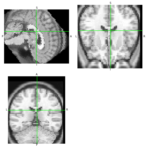
The outputs of AFNI and NiTransforms should be consistent:

moved_afni.orthoview()
moved_oblique.orthoview()

<OrthoSlicer3D: (57, 67, 56)>

WAT?? O_O the two images do not match. Let’s look at the affines of each.

moved_afni.affine[:3, ...].round(2), moved_oblique.affine[:3, ...].round(2)

(array([[  2.75,  -0.  ,  -0.  , -86.7 ],
        [ -0.  ,   2.75,  -0.  , -72.74],
        [  0.  ,   0.  ,   2.75, -99.19]]),
 array([[ 2.740e+00,  0.000e+00,  2.700e-01, -8.670e+01],
        [ 5.000e-02,  2.700e+00, -5.400e-01, -7.274e+01],
        [-2.700e-01,  5.500e-01,  2.680e+00, -9.919e+01]]))

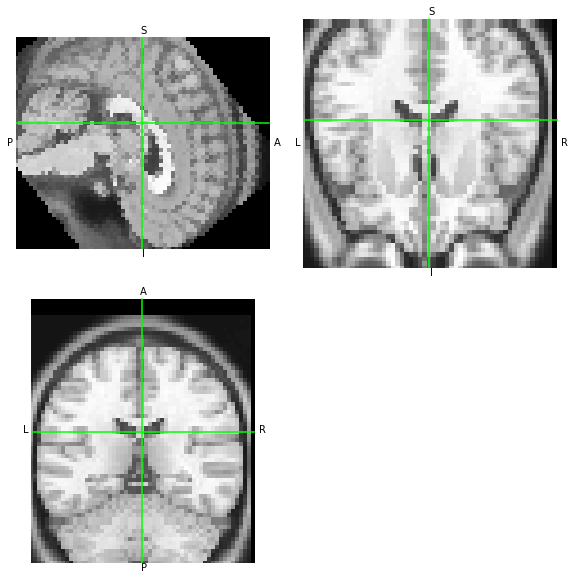
We can see that AFNI has generated a dataset without obliquity. If both tools are generating the same data at the output with only a difference in the orientation metadata, then both data arrays should be similar – let’s overwrite the metadata and compare visually:

moved_oblique.__class__(
    np.asanyarray(moved_afni.dataobj, dtype="uint8"),
    moved_oblique.affine,
    moved_oblique.header,
).orthoview()
moved_oblique.orthoview()

<OrthoSlicer3D: (57, 67, 56)>